Fast conversion of bitmaps to SVG

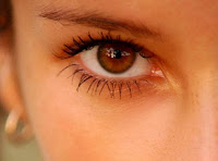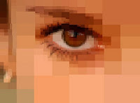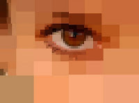
The image on the left is the 600x446-pixel "original" RGB image; the copy on the right has been tiled into 6706 solid-filled rectangles. See text for discussion.

Conversion of bitmapped images (*.jpg, *.gif, etc.) to vector format (Postscript, SVG) is, in general, a Difficult Problem. In some ways, it's not unlike trying to convert spoken text (in the form of *.mp3 audio) to ASCII. Well okay, maybe it's not that bad, but it's gnarly. You're trying to parse precise geometric shapes out of an ensemble of intensity samples. It's not at all obvious how to do it. Finding a fully general algorithm for describing an arbitrary bitmap as an ensemble of vector-drawable shapes is vexingly difficult. You might as well try to reassemble Yugoslavia.

You have to admit, though, it'd be darned handy to be able to transcode a bitmap image into (say) some flavor of XML (such as SVG). Unlike binary formats, XML is wire-protocol-friendly, queryable at the element and attribute level, transformable using XSLT (and/or E4X, or other technologies), human-readable (bwahhh-ha-ha . . .), and highly compressible. Converting JPEG to XML would open the door (potentially) to many interesting operations. Imagine running XPath queries against images to find specific areas of interest, or morphing one image into another using XSLT.

While there is obviously no one right way to proceed, I'd like to propose an approach to the problem (the problem of how to transcode bitmaps to SVG) based on quadtree decomposition of an image into polygons -- rectangles, in particular. It's possible to apply the same approach using triangles as primitives, instead of rects, or spline patches for that matter, but rectangles offer some noteworthy advantages. Most images are rectangles to begin with, of course, and parsing them into smaller (but adjoining) rects is a natural thing to do. Once parsed, rects allow a relatively compact representation; and at render-time, not many solid shapes are easier or faster to draw.

We have the considerable advantage of being able to start from the perspective of seeing a bitmapped image as just a grid of one-by-one rectangles (known as pixels). Two adjoining pixels of the same color become a 1x2 solid-color rect, four adjoining identical pixels become a 2x2 or 1x4 rect, and so on. Surely we can parse out the "naturally occurring" solid-filled rects within a pixel lattice? Those rects are instantly vector-drawable.

If we do this, we'll get what we get -- probably a very small handful of accidental finds. But we can do better, if (through preprocessing) we quantize pixel values in such a way as to force nearly-equal pixels to be equal in value. This will cause the appearance of a higher percentage of solid-color rects within a bitplane. Of course, when we're done, there's still no guarantee we will have covered the entire visual plane with rects (unless, as I say, we count individual pixels as 1x1 rects). Nevertheless, it's an interesting strategy: Force adjoining almost-equal pixels to be equal in value, then aggregate them into solid-color rects. Deal with the leftovers later.

At the extreme, we can look at the entire image as being a collection of pixels that are nearly equal in value. There is actually considerable variance in pixels, of course (unless the image is truly not very interesting). But what we might do is quantify the variance in some way, and if it exceeds a threshold, divide the image into daughter rects -- and begin again. We know that eventually, if we keep subdividing, we'll get to individual pixels (1x1 rects) that have zero variance within themselves. By this sort of strained logic we might convince ourselves that there should be less variance in small rects than in large ones, as a general trend.

Let me get right to it and propose an algorithm. (Listen up.) Start by considering a rectangle covering the whole image. Going pixel by pixel, calculate some variance measure (such as root-mean-square variation from average) for all pixels, for the whole region. If the variance is low (lower than some arbitrary limit), consider all pixels within the region to be equal; define the region as a rect of color Argb (representing the arithmetic average of the pixel values). If the variance exceeds an arbitrary threshold, subdivide the image. Specifically, subdivide it into four (generally unequal) rects.

To determine where to subdivide, calculate the "center of gravity" of the parent rect. A pixel's lightness or darkness, multiplied by its position vector, gives its moment-in-X and moment-in-Y. Add all the X moments together (and the Y moments). Divide by the number of pixels. The result is the visual center of the region. That's where you divide.

Repeat the procedure on newly created rectangular regions. Any regions with low variance can be rendered as a solid-color rect; the other regions are subdivided, and the algorithm continues until reaching individual pixels, or until every region larger than a pixel was successfully encoded as a rect.

This general technique is known as quadtree subdivision and it lends itself well to recursive implementation. You're not likely to get into stack-overflow problems with it, because with four times as many rects at each recursion cycle, you'll have created (potentially) over 1000 rects in just 5 cycles. Ten levels deep, you've created a million rects. Better start worrying about heap, not stack.

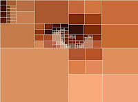
A demonstration of the technique can be seen below. The image on the left was created using a fairly "insensitive" variance threshold of 29 (meaning that subdivision did not occur unless a region had an RMS variance of at least 29, out of a possible range of pixel values of 0..255). Because subdivision happened infrequently, only in the very noisiest of pixel regions, smaller rects tended to cluster in areas of high detail (high variation in pixel intensities), such as around the edges of the iris and eyelashes. The image on the right shows that with the RMS threshold set lower (at 22), we get more detail -- about 300 rects total. (White outlines around the rects have been omitted on the right image.)

The image on the left has been parsed into 136 solid rectangles (with white outlines for illustrative purposes) using the recursive quadtree decomposition described in the text. Notice how subdivision into smaller rectangles tends to coincide with areas of high detail. The image on the right has been parsed into 334 rects.

The algorithm is tunable in a couple of ways. The most obvious way is via the variance-cutoff parameter. If the variance threshold is set low, it means that the slightest bit of "noise" in a given region will trigger subdivision of the region (and continued operation of the algorithm). However, we have to stop subdividing before reaching individual pixels. So another tuning variable is the minimum tile size.



The image on the left is a collage of 790 solid-filled rectangles. At a rect count of 2209, the image on the right is starting to have a bitmap-like feel.

The code that produced these images consists of 200 lines of JavaScript (shown below) and another 200 lines of Java utility routines (in a class called ImageUtilities: see further below). In addition to that, you need the ImageMunger Java application that I described in yesterday's post (yet another 200 lines or so of Java). First, the JavaScript:

// tiles.js
// Kas Thomas
// 23 January 2010
//
// Public domain.
//
// Note: For this to work, you need the ImageMunger
// Java app at http://3.ly/UBp
// You also need the ImageUtilities class described
// at the same blog.

// ------------------ RECURSIVE SUBDIVISION -------------------
function quadRecurse( ar, rect ) {

   if ( !isDivisible( rect ) ) {
           ar.push( rect );
           return;
   }

   var newRects = quadDivide( rect ); // partition rect

   for (var i = 0; i < newRects.length; i++)  // size check
   if (newRects[i][2] < 1 || newRects[i][3] < 1) {
           ar.push(rect);
           return;
   }

   for (var i = 0; i < newRects.length; i++) // recurse on each new rect
   quadRecurse( ar, newRects[ i ] );
}

function quadDivide( rect ) {

   var pixArray = getPixArrayFromRect( rect );

   // Get the visual "center of gravity" of the image
   var cg = Packages.ImageUtilities.getCG( pixArray, rect[2] );

   cg[0] =  (cg[0] + .5) * .5;
   cg[1] =  (cg[1] + .5) * .5;
   cg[0] = 1.0 - cg[0];
   cg[1] = 1.0 - cg[1] ;

   var centerx = ( (cg[0] * rect[2]) & 0xffff);
   centerx += rect[0];
   var centery = ( (cg[1] * rect[3]) & 0xffff);
   centery += rect[1];

   var widthToCenterx  = centerx - rect[0];
   var heightToCentery = centery - rect[1];

   var rect1 = [ rect[0], rect[1], widthToCenterx, heightToCentery ]; // UL
   var rect2 = [ rect[0], centery, widthToCenterx, rect[3] - heightToCentery]; // LL
   var rect3 = [ rect[0] + widthToCenterx, rect[1], rect[2] - widthToCenterx, heightToCentery ]; // UR
   var rect4 = [ rect[0] + widthToCenterx, centery, rect[2] - widthToCenterx, rect[3] - heightToCentery ]; // LR

   return [ rect1, rect2, rect3, rect4 ];
}

// -------------- divisibility ----------------
function isDivisible( rect ) {

   if (rect[2] < WIDTH_THRESHOLD || rect[3] < HEIGHT_THRESHOLD)
   return false;

   var pixArray = getPixArrayFromRect( rect );
   var rms = Packages.ImageUtilities.getRMSError( pixArray );

   if (rms < RMSERROR_THRESHOLD)
   return false;

   return true;
}

function getPixArrayFromRect( rect ) {

   var sub = Image.getSubimage( rect[0],rect[1],rect[2],rect[3] );
   return sub.getRGB(0, 0, rect[2], rect[3], null, 0, rect[2]);
}

// -------------------- RENDER ---------------------------------------
function render( ar ) {

   var g2d = Image.createGraphics();
   var r = null; var sub = null; var pixels = null;
   var color = null;

   for (var i = 0; i < ar.length; i++) {
           r = ar[i];
           if (r[2] <= 0) continue; // r[2] = 1;
           if (r[3] <= 0) continue; //r[3] = 1;

           pixels = getPixArrayFromRect(r);
           color = Packages.ImageUtilities.getAverageAWTColor( pixels );

           g2d.setPaint( color  );
           g2d.fillRect( r[0], r[1], r[2], r[3] ); // FILL SOLID

           if (OUTLINES == true) {
                   g2d.setColor( java.awt.Color.WHITE );
                   g2d.drawRect( r[0], r[1], r[2], r[3] );
           }
   }

   Panel.updatePanel();
}

// -------------------- WRITE SVG ----------------------
function writeSVG( preamble, destfile, ar ) {
   var r = null; var pixels = null; var awt = null;
   var color = null;

   var output =
   '<?xml version="1.0" encoding="UTF-8" standalone="no"?>'+
   '\n<!DOCTYPE svg PUBLIC "-//W3C//DTD SVG 20010904//EN" ' +
   '"http://www.w3.org/TR/2001/REC-SVG-20010904/DTD/svg10.dtd">' +
   '<svg xmlns="http://www.w3.org/2000/svg" ' +
   'xmlns:xlink="http://www.w3.org/1999/xlink" ' +
   'viewBox="0 0 640 480" ' +
   'xml:space="preserve" ' +
   'width="680px" ' +
   'height="560px">';

   output += "<g transform=\"scale(.85)\">";

   for (var i = 0, r = null; i < ar.length; i++) {
           r = ar[i];
           pixels = getPixArrayFromRect(r);
           awt = Packages.ImageUtilities.getAverageAWTColor( pixels );

           color = awtColorToHex( awt );

           output += outputSVGRect( mainArray[i], color );
   }
   output += "</g>";
   output += "\n</svg>";

   // write output to file
   Packages.ImageUtilities.saveStringToFile(output, destfile);
}

function intToHex( num ) {
   num *= 1;
   hexStr = '000000' + (num).toString(16);
   while ( hexStr.length > 6)
   hexStr = hexStr.substring(1);

   return "#" + hexStr;
}

function awtColorToHex( awt ) {
   var theInt = (awt.getRed()<<16)|(awt.getGreen()<<8)|awt.getBlue();

   return intToHex( theInt );
}

function outputSVGRect( r, color ) {

   var str = "<rect x=";
   str += "\"" + r[0] + "\" ";
   str += "y=\"" + r[1] + "\" ";
   str += "width=\"" + r[2] + "\" ";
   str += "height=\"" + r[3] + "\" ";
   str += "fill=\"" + color + "\" ";
   str += "stroke=\"" + color + "\" ";
   str += "/>\r";

   return str;
}

// ---------- Main work routine ------------
// Usage:
//
//   doQuadding( 10, 6, "svg", "C:/test1.svg" );
//   (writes output to an SVG file)
//
// or:
//
//   doQuadding( 11,4, "preview", null );
//   (renders image in JFrame)

function doQuadding( rms, sizeLowLimit, mode, dest ) {

   if (Image == null) {
           java.lang.System.out.println("Nothing to do; no source image." );
           return;
   }
   w = Image.getWidth(); h = Image.getHeight();
   mainRect = [ 0,0,w,h ];
   mainArray = new Array();

   RMSERROR_THRESHOLD = rms;
   WIDTH_THRESHOLD = HEIGHT_THRESHOLD = sizeLowLimit;

   quadRecurse( mainArray, mainRect );  // *** RECURSE ***

   java.lang.System.out.println("Total rects: " + mainArray.length );

   if (mode.toLowerCase().indexOf("preview") != -1) {
           java.lang.System.out.println("  rendering... " );
           render( mainArray );
   }
   if (mode.toLowerCase().indexOf("svg") != -1) {
           java.lang.System.out.println("  writing... " );
           writeSVG( "c:/temp/svgStub.txt", dest, mainArray);
           java.lang.System.out.println("DONE.");
   }
}

OUTLINES = false;
var start = 1 * new Date;
//  Actually call the entry point (begin processing):
doQuadding( 8,6, "preview", null );
//  doQuadding( 8,6, "svg", "c:/temp/test86.svg" );
var end = 1 * new Date;
java.lang.System.out.println("Finished in " + (end-start) +
" milliseconds");

To use this file, give it a name like tiles.js, then run ImageMunger (the Java app I described in yesterday's post) from the command line, passing it the name of the image you want to modify, and the name of the script file:

> java ImageMunger myImage.jpg tiles.js

The entry point for the script is doQuadding(), which you can call with a 3rd argument of "svg" if you want to write output to a Scalable Vector Graphics file. Otherwise pass a 3rd arg of "preview" and ImageMunger will simply render the transformed image to a JFrame.

The script makes reference to a number of utility routines written in Java. The utility routines are in a class called (what else?) ImageUtilities, as follows. The routines should be fairly self-explanatory.

import java.io.BufferedReader;
import java.io.File;
import java.io.FileOutputStream;
import java.io.FileReader;
import java.io.IOException;
import java.io.OutputStream;

/*
ImageUtilities.java

Kas Thomas
23 January 2010
See http://3.ly/UBp and subsequent posts.
*/

public class ImageUtilities {

  public static void saveStringToFile( String content,
  String outpath ) {

          OutputStream out = null;
          try {
                  out = new FileOutputStream(outpath);
                  out.write(content.getBytes());
          } catch (IOException e) {
                  System.out.println("Couldn't save to " + outpath);
                  e.printStackTrace();
          } finally {
                  try {
                          if (out != null)
                          out.close();
                  } catch (IOException e1) {
                          e1.printStackTrace();
                  }
          }
  }

  // Get the visual center-of-gravity of a pixel array.
  // Pass the array and the raster width.
  public static double [] getCG(int [] pix, int w) {

          double intensity = 0;
          int red = 0;
          int green = 0;
          int blue = 0;
          double [] cg = { 0,0 };
          double averageIntensity = 0;
          int pvalue = 0;

          for (int i = 0; i < pix.length; i++ ) {
                  pvalue = pix[i];
                  red = ((pvalue >> 16) & 255);
                  green = ((pvalue >> 8) & 255);
                  blue = pvalue & 255;
                  intensity = ((double)(red + blue + 2 * green))/1024.;
                  averageIntensity += intensity;
                  cg[0] += intensity * (i % w);
                  cg[1] += intensity * (i / w);
          }

          cg[0] /= averageIntensity;
          cg[1] /= averageIntensity;

          cg[0] /= w;
          cg[1] /= pix.length/w;
          return cg;
  }

  public static double getRMSError(  int [] pix ) {

          double accumulator = 0;
          double diff = 0;
          double aveIntensity = 0;
          double rms = 0;
          int len = pix.length;

          for (int i = 0; i < len; i++) {
                  aveIntensity += (double)((pix[i] >> 8) & 255);
          }

          aveIntensity /= len;

          for (int i = 0; i < len; i++) {
                  diff = (double)((pix[i] >> 8) & 255) - aveIntensity;
                  accumulator += diff * diff;
          }

          rms = accumulator/len;

          return Math.sqrt(rms);
  }

  public static java.awt.Color getAverageAWTColor( int [] input ) {

          int ave = getAverageColor( input );
          int red = (ave >> 16) & 255;
          int green = (ave >> 8) & 255;
          int blue = ave & 255;
          return new java.awt.Color(red,green,blue);
  }

  public static int getAverageColor( int [] input ) {

          int red = 0;
          int green = 0;
          int blue = 0;
          int pvalue = 0;
          int averageRed = 0;
          int averageGreen = 0;
          int averageBlue = 0;

          int len = input.length;

          for (int i = 0; i < len; i++) {

                  pvalue = input[i];
                  red = ((pvalue >> 16) & 255);
                  green = ((pvalue >> 8) & 255);
                  blue = pvalue & 255;

                  averageRed += red;
                  averageGreen += green;
                  averageBlue += blue;

          }

          averageRed /= len;
          averageGreen /= len;
          averageBlue /= len;

          return (averageRed << 16) | (averageGreen << 8) | averageBlue;
  }

  public static double getIntensity( int pvalue ) {

          int red = ((pvalue >> 16) & 255);
          int green = ((pvalue >> 8) & 255);
          int blue = pvalue & 255;

          double intensity = red + blue + 2 * green;

          return intensity/1024.;
  }

  public static double getIntensity( java.awt.Color c) {

          int intvalue = c.getRed() << 16;
          intvalue += c.getGreen() << 8;
          intvalue += c.getBlue();
          return getIntensity( intvalue );
  }

  public static java.awt.Color getAWTColor( int pvalue ) {

          int red = ((pvalue >> 16) & 255);
          int green = ((pvalue >> 8) & 255);
          int blue = pvalue & 255;

          return new java.awt.Color(red,green,blue);
  }

  public static double getRMSE( int [] pix1, int [] pix2) {

          double rms = 0;
          double accum = 0;
          double intensity1 = 0;
          double intensity2 = 0;
          double tmp = 0;

          if (pix1.length != pix2.length) {

                  System.out.println("Arrays are not the same size.");
                  return rms;
          }

          for (int i = 0; i < pix1.length; i++) {
                  intensity1 = getIntensity( pix1[i] );
                  intensity2 = getIntensity( pix2[i] );
                  tmp = intensity1 - intensity2;
                  tmp *= tmp;
                  accum += tmp;
          }

          rms = accum/pix1.length;  // the mean of the squares
          return Math.sqrt( rms );  // root mean square
  }
}

Even though the main routine is in JavaScript, the overall processing runs quickly. The algorithm executes in near-linear time and can output around 5000 rectangles per second (to screen, that is; disk I/O not included).

Projects for the future:

• Write gradient-filled rects instead of solid-filled rects, choosing the gradient endpoint colors in such a way as to minimize the differences between the output and the original image.
• Given two SVG images, each an ensemble of rects (preferably equal in number), write a transformation routine that morphs one image into the other via transformations to the individual rects (and their colors). Store the second image as simply an ensemble of transformations (no rects). The first image provides the "reference rectangles" that will be transformed.
• Write a public key image-encryption routine based on the foregoing notion, such that Image A becomes a key that someone can use to encrypt Image B, with private-key Image C unlocking B.
• Instead of writing an SVG image as an ensemble of individual rects, write it as one rect that is repeatedly resized and repositioned via successive affine transformations.
• Encrypt an image using the above technique (rewrite one rect many times through transformation) in concert with matrix hashing. Write an SVG image-encryption routine whose difficulty of decryption depends on the non-commutative nature of matrix multiplication and the numerical instability of inverted matrices.
• Write a "chunky JPEG" routine that essentially uses the quadtree decomposition to chunk the image prior to discrete cosine transformation, instead of using the (canonical JPEG) 8x8 chunking.
• [ Insert your own idea here! ]